How to give them the Cohen's d
Cohen's d is one of the most popular measures of effect size out there. It happens sometimes that Cohen's d is not accurately translated into our intuitions of how relevant soething is. Here I will explain it with a few charts.
Cohen's d measures effect size, which a standarised measure of the difference between two distributions. In the case of Cohen's d,
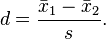
That's the difference between two distribution's means, over a pooled standard deviation, and it looks like this: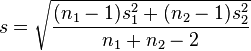
Let's look at some examples.
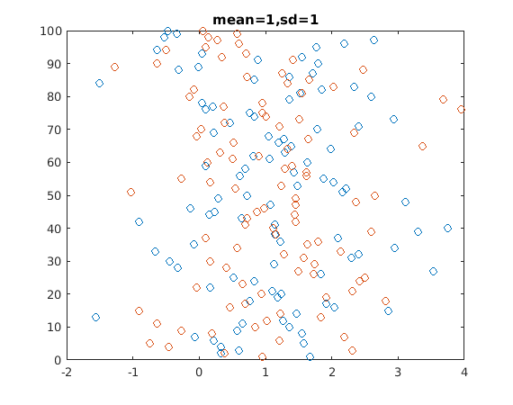
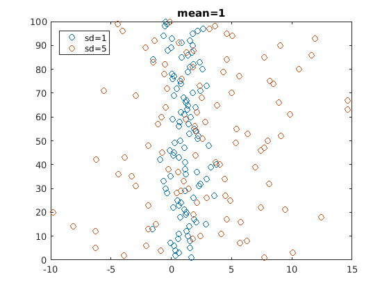
First, here are 100 draws from two normal distributions (100 from each). Both have mean one, and a standard deviation of one. Given this, Cohen's d is zero. This picture is here just to give you a feel of what draws from a normal distribution look like.
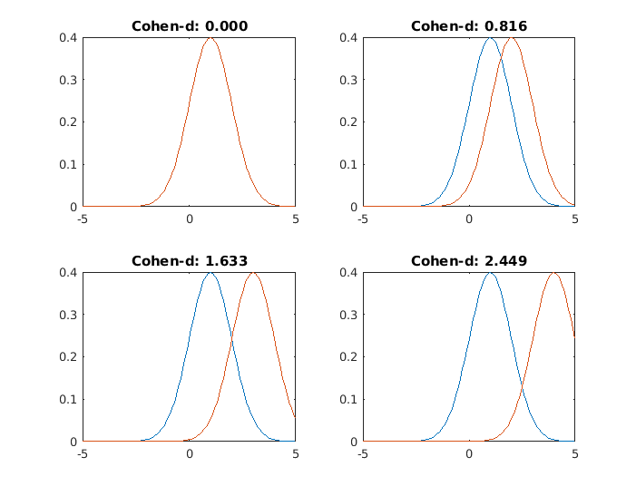
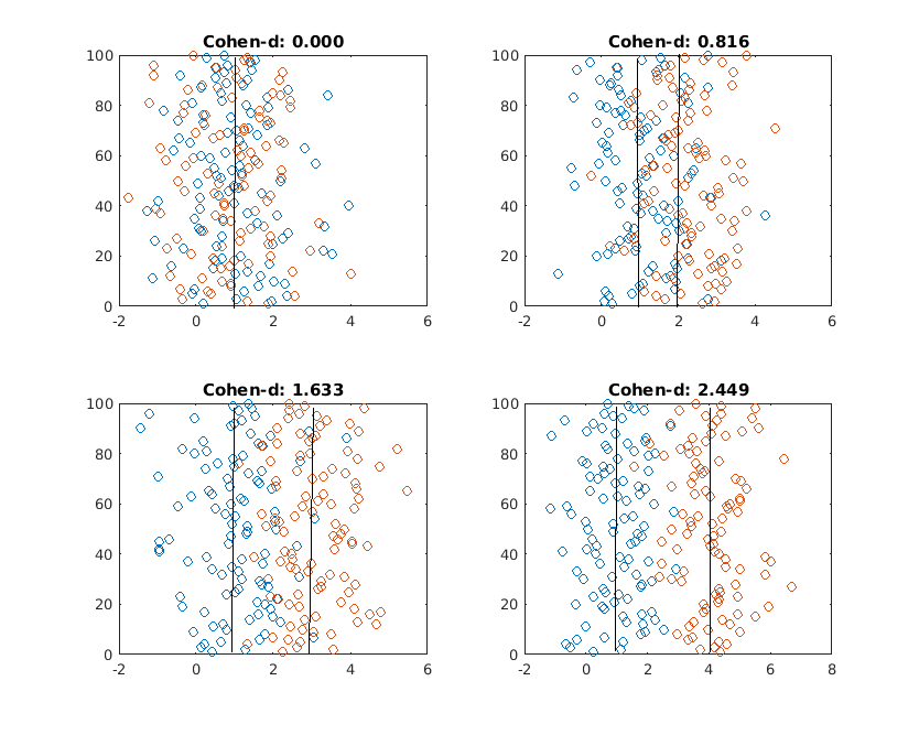
My next chart has, again, mean=1 normal distributions, but the standard deviations change. The blue distribution's is always 1, while for the orange one, it is 1,2,3 and 4 in each of the charts. In all of then, Cohen's d is zero, as the means are equal.
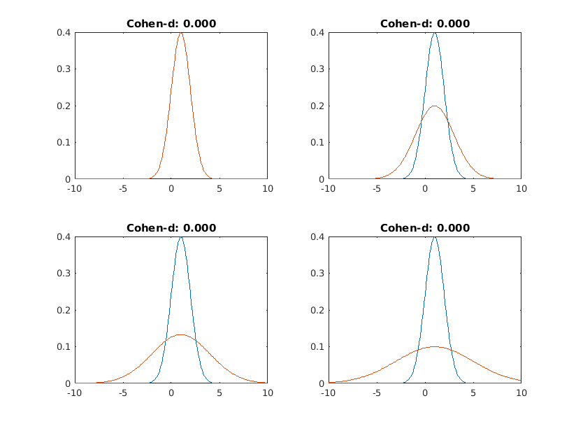
If we look at individual draws, it's obvious what's happening here: while if you just take many observations you see no difference in the mean, if you set a cutoff point and want to observe the tails of the distribution, you will find that the lowest and highest values correspond to the orange distribution. So if there are Orange people and Blue people, you would only find geniuses and mentally retarded among the Oranges, while far more blues would be average.
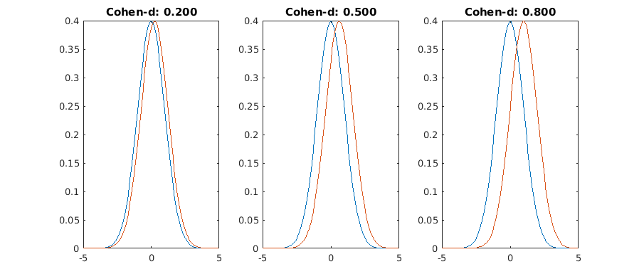
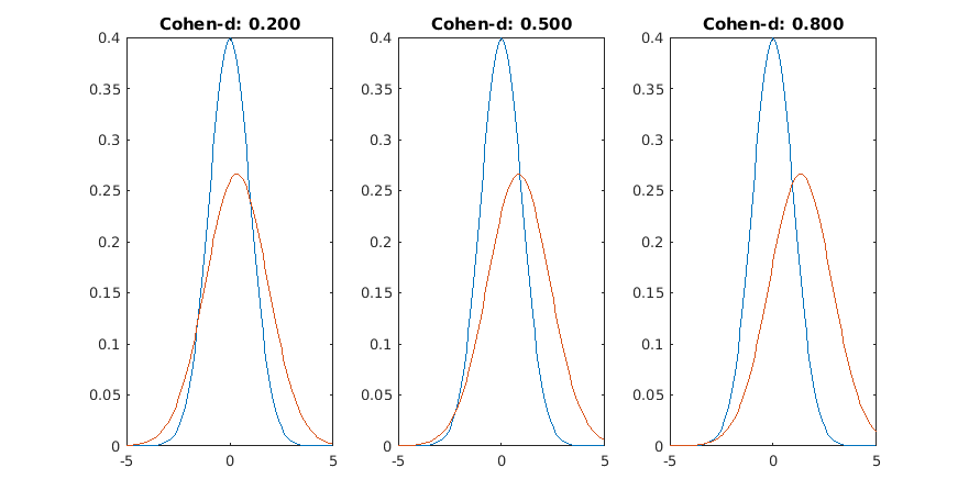
Now, we repeat the procedure for two distributions with the same standard deviation (sd=1), and different means (1,2,3,4)
How to interpret Cohen's d?
Here they say that 0.2 is small, 0.5 is medium and 0.8 is large, and this criterion is pretty much followed everywhere.
Yes, they don't look much different now. Here's with different standard deviations (sd=1, sd=1.5)
Another measure we can consider to get a better feel of Cohen's d is to think of the expected distance between two draws from the same distribution, vs the expected distance between one draw from each distribution. This second value is just given by the difference between the means. The first value can be obtained from here as twice the standard deviation over the square root of pi. For a sd=1 distribution, this is 1.128. So if the difference between the means is less than 1.128, two randomly chosen Blues (sd=1,m=0) will be more different than the difference between the average Blue (sd=1,m=0) and the average Orange (sd=1, m=1).
Translating this into Cohen's d, it means that even if you have large effect sizes (1.0), it will still be the case that the differences between two draws from one distribution will be larger than the distance between the averages of the two distributions.
To finish, two practical applications.
The first one is female-male height in Spain in 1980 (Garcia y Quintana-Domeque, 2007). Everyone has experience with this one:
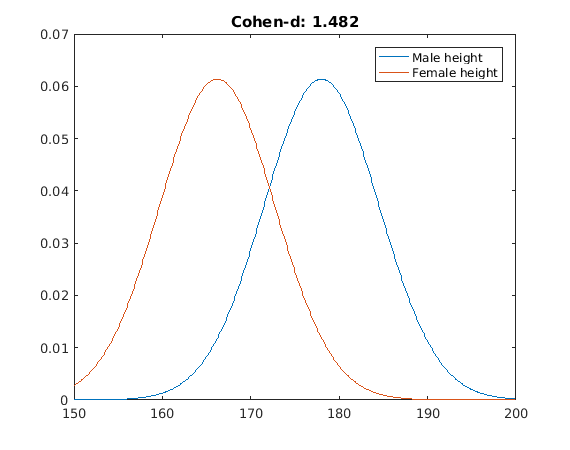
Here,the probability of a random man being taller than a random woman is around 0.86. 93% of males will be above average female height, and there will be a 45% overlap between both groups.
Next example: male-female differences regarding career choice. From here, the difference between male-female preferences regarding engineering can be said to be described by d=1 (A randomly picked male will be more interested in engineering than a randomly picked female, with 0.76 probability). The same for medical services and social sciences is d=-0.4 (Same as before, 0.61 probability) and d=-0.33 (0.58 probability), respectively. Note that these Cohen d's add up, so to speak. If women are less likely to like being engineers and more likely to like being social scientists, this two effects will alter the career distribution by more than you would expect from d=1. It is then important to look at the context in which a statistical claim is made.
Just given this, the authors of one study cited estimate how many men and women there will be in each field, and compare it to the actual numbers:
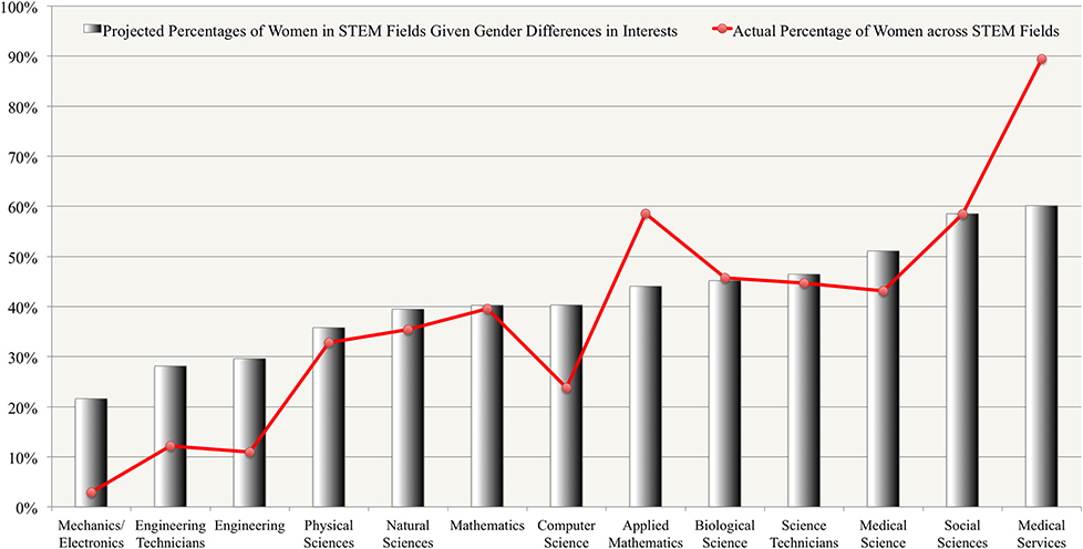
This just assumes women and men are equal in everything else. From this, women are underrepresented in engineering, and overrepresented in medical services, and this deviation is not accounted for by interests. Other factors mentioned are different work-life balance preference, gender stereotyping, and implicit biases in employers' selection proceses, and differences in skills (women who have high mathematical skills are more likely than men to also have high verbal skills. So these men will go to become engineers, while women have more options open)
Conclusion
Cohen's d is the most common, and perhaps the most useful, way of expressing effect sizes. Understanding it is a bit problematic given that unlike other statistical measures like R², it doesn't go from 0 to 1 (Or -1 to 1) with 0 meaning no effect and 1 meaning maximum effect. Cohen-d's go from 0 to infinity (in absolute value). Understanding it gets more complicated when you notice that two distributions can be very different even if they have the same mean. I would then recommend trying to picture the actual distributions when thinking about Cohen's d, or even build a simple model to see what predictions can we make from the observed differences, like it was done above for career choice.
Comments